Statistics in the Laboratory: The Limit of Detection

Featured Article

The phrase “limit of detection” sounds so simple, yet it leads to one of the biggest, murkiest, most frustrating swamps in the statistical literature. All the organizations in all the towns in all the world took it upon themselves to define, redefine, and re-re-redefine the phrase. This resulted in hundreds of definitions for “limit of detection.” In 1968, Lloyd Currie decided enough was enough, and published his famous paper clarifying limits of detection and related topics.¹ Richard Lindstrom said it best:²

Until Lloyd Currie’s paper … was published, there was enough inconsistency in the definition of “detection limit” to conceal a great deal of disagreement. In just over seven pages, this tightly written communication established a high level of uniformity in answering these questions. The paper contains fundamental information that has made it influential far beyond its size, and it is rich enough to be discussed actively in e-mail newsgroups [now nearly 50] years later. This is surely one of the most often cited publications in analytical chemistry.

In this and the next two columns, we’ll use Currie’s approach (with slightly different symbols) to discuss the limit of detection (L_D; Currie uses L_C), the minimum consistently detectable amount (MCDA, related to Currie’s L_D), and the limit of quantitation (L_Q). Then we’ll see how John Mandel’s definition of sensitivity allows a meaningful comparison of these three quantities for the “apples and oranges” of disparate units for different analytical methods (e.g., peak area in chromatography, ion intensity in mass spec).

Detection limits have been discussed previously in American Laboratory, most notably in the acclaimed “Statistics in Analytical Chemistry” series by David Coleman and Lynn Vanatta, installments 26 (https://www.americanlaboratory.com/913-Technical-Articles/1254-Part-26-Detection-Limits-Editorial-Comments-and-Introduction/), 28–30 (https://www.americanlaboratory.com/914-Application-Notes/1094-Part-28-Statistically-Derived-Detection-Limits/, https://www.americanlaboratory.com/914-Application-Notes/1095-Part-29-Statistically-Derived-Detection-Limits-continued/, https://www.americanlaboratory.com/914-Application-Notes/1096-Part-30-Statistically-Derived-Detection-Limits-concluded/), and 32–34 (https://www.americanlaboratory.com/914-Application-Notes/1104-Part-32-Detection-Limits-Via-3-Sigma/, https://www.americanlaboratory.com/914-Application-Notes/1105-Part-33-Detection-Limits-via-3-Sigma-Concluded/, https://www.americanlaboratory.com/914-Application-Notes/1106-Part-34-Detection-Limit-Summary/) from June 2007 through May 2009. The work of Currie has been the basis of an oft-cited paper by Hubaux and Vos.³

Spoiler alert 1: Many persons think the limit of detection (often mistakenly called the “sensitivity”) is the smallest amount of analyte that can be detected reliably—that’s going to be the MCDA, discussed in the next column. The limit of detection L_D (discussed in this column) and the limit of quantitation L_Q (discussed in the column after next) have to do with the signal strength (e.g., peak area, ion intensity). Be prepared to adjust your focus.

Spoiler alert 2: There are no universal values for these things. You (the analyst) and your client have to consider the application of your measurement method and use an acceptable false positive risk α, an acceptable false negative risk β, and your egos to set L_D, MCDA, and L_Q, respectively. Currie’s paper provides the structure for making the connections.

Figure 1 – A realistic calibration relationship with non-zero intercept μ_b and noise σ_b.

Figure 1 shows a realistic calibration relationship between the amount of analyte (the horizontal x-axis) and the signal obtained from the measurement method (the vertical y-axis). In this figure, each vertical line segment represents one measurement—the line begins at the calibration relationship and extends out to the measured value. Statistical analysis (usually linear least squares) can be used to obtain the best fit of a two-parameter (slope and intercept) straight line to these noisy data. The y-intercept of the calibration line will be called the true mean of the blank μ_b, where a blank is a sample containing no analyte. The standard deviation of the blankσ_b can be obtained from the variation of the data points about the fitted calibration line at small amounts of analyte. Alternatively, both μ_b and σ_b can be obtained from repetitive measurements of a blank sample. In this column we’ll assume that the uncertainties in estimating μ_b and σ_b are sufficiently small that we may represent them as population parameters. For generality, the calibration relationship shown in Figure 1 has a non-zero μ_b.

Figure 2 – The false positive risk α of setting L_D equal to μ_b.

Figure 2 shows the results of multiple measurements of a blank. Note that the horizontal x-axis is now the measurement number, not the amount. The Gaussian distribution in the new panel at the left summarizes the measurements—the Gaussian is centered at μ_b and has a standard deviation of σ_b.

Here’s the way the game is played. Given a limit of detection L_D, if y represents the measured signal for a sample containing an unknown amount of analyte, the rules are:

if y ≥ L_D, analyte is said to be detected (present)

if y ≤ L_D, analyte is said to be not detected

Not detected doesn’t necessarily mean absent; it just means that if there is any analyte present, there isn’t enough of it to give a signal strong enough to say that it’s been detected.

You get to decide what value you’re going to use for L_D. Let’s look at a couple of possibilities.

Suppose you decide to set the limit of detection L_D equal to the true mean of the blank μ_b as shown in Figure 2. If you then make multiple measurements on a blank, half the time you’ll get a signal y that’s less than L_D (the green measurements) and conclude that analyte has not been detected. So far, so good: there is no analyte to detect. But half the time you’ll get a signal y that’s greater than L_D (the red measurements) and conclude that analyte has been detected. This does not represent the truth. This is a positive statement (“analyte is present”) that’s clearly false; in fact, it’s called a false positive, and in this case the false positive risk α is equal to 0.5 (half the measurements lie in the red part of the Gaussian).

For most applications, α = 0.5 is probably an unacceptable false positive risk. Consider a drug-testing laboratory. If L_D = μ_b for each drug test, then a non-drug user stands a 50% chance of being wrongly accused of having a specific drug in his or her body. It’s worse if k drugs are being tested at the same time. Remember α_EW, the overall “experiment-wise” risk of making at least one false positive statement:

                      (1)

For k = 10 simultaneous drug tests, the overall risk of getting at least one false positive result is 0.9990234375, or greater than 99.9%. This means that if 1000 totally clean applicants were each tested for a battery of 10 illicit drugs, it is expected that 999 of them would be falsely accused of having one or more of those drugs in their bodies. Are you beginning to see that the false positive risk α should be appropriate for the application? You and your client need to decide what α should be, and then adjust L_D appropriately.

So how do you do that? Let’s say you get together with your client and decide that an acceptable α_EW would be 0.005 (0.5%; now only 5 nailed out of 1000 innocents … but you’ll let them take the drug test again to further decrease their chances of being wrongly accused). You can rearrange Eq. (1) to give

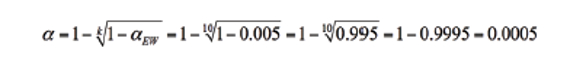(2)

Looking at a statistical table of z-values, you find that you need to go out about 3.3 standard deviations from the mean to exclude this fractional area α from one tail of a Gaussian curve. This is shown in Figure 3, where L_D = μ_b + 3.3×σ_b. If the sample contains no analyte, then the probability of getting a measured signal greater than μ_b + 3.3×σ_b is 0.0005; thus, the risk of making a false positive statement that analyte has been detected is 0.05%, 1/20th of one percent.

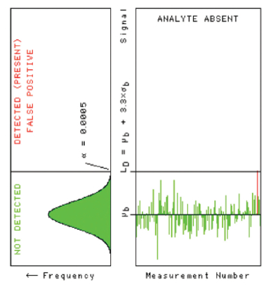Figure 3 – The false positive risk α of setting L_D equal to μb + 3.3×σ_b.

It’s curious that this value of L_D = μ_b + 3.3×σ_b is often found in the literature. Each application should require a different false positive risk, so why do so many applications seem to require 1/20th of one percent as the false positive risk? It doesn’t make sense. But here’s some history: someone once asked Sir Ronald A. Fisher (for whom the F test was named) what the false positive risk should be for scientists trying to discover the laws of the universe, and he said something like, “Oh, one time in twenty would be OK, I guess,” which gives us our common 95% level of confidence.⁴ I can only speculate that to some persons, “one-twentieth of one percent” sounds like something Fisher might recommend; it sounds kind of scientific, somehow.

You and your client shouldn’t automatically adopt a value of 0.0005, or 0.005, or any other specific value for α. Think about your application and set an appropriate value for the false positive risk. Then you can use α, μ_b, σ_b, and a z-table to find the corresponding value for L_D.

Figure 4 – The concept of a false negative.

Let’s go back and consider again the statement that “not detected doesn’t necessarily mean absent; it just means that if there is any analyte present, there isn’t enough of it to give a signal strong enough to say it’s been detected.” Look at Figure 4. In this example, with L_D = μ_b + 3.3×σ_b, the probability of a false positive is 0.0005 for a blank. For a sample that contains just a tiny amount of analyte (moving to the right in the figure), the truth is that analyte is present, but the probability of not detecting it is very large (a bit less than 0.9995, but still very large). This is the false negative risk β. Clearly, the false negative risk depends on the amount of analyte actually present.

In the next column, we’ll explore the relationship between the false negative risk and the amount of analyte. This will lead us to the minimum consistently detectable amount, the MCDA.

Remember: the limit of detection L_D is on the vertical signal axis of a calibration plot; the minimum consistently detectable amount MCDA will be on the horizontal amount axis.

References

1. Currie, L.A. Limits for qualitative detection and quantitative determination: application to radiochemistry. Anal. Chem.1968, 40(3), 586–593.
2. Lindstrom, R.M. In Lide, D.R., Ed. A Century of Excellence in Measurements, Standards, and Technology: A Chronicle of Selected NBS/NIST Publications, 1901-2000; NIST Special Publication 958, 2001.
3. Hubaux, A. and Vos, G. Decision and detection limits for linear calibration curves. Anal. Chem.1970, 42(8), 849–855.
4. Moore, D.M. Statistics: Concepts and Controversies; Freeman: San Francisco, CA, 1979.

Stanley N. Deming, Ph.D., is an analytical chemist masquerading as a statistician at Statistical Designs, El Paso, TX, U.S.A.; e-mail: [email protected]; www.statisticaldesigns.com